From P-Code to GNN: Extracting Binary Code Semantics

Original text: "From P-Code to GNN: extract binary code semantics" — Samuel Hangouët, Quarkslab (13 August 2026). Library: github.com/quarkslab/pcode_graph (MIT). Code, tables and figures below are reproduced verbatim with attribution captions.

Same C function, five compilers, six ISAs: the graph should still be the same dish.

Kitchen: -Oz and -O0 are two cookbooks for the same stew. Count the words and you think they are different meals.

Executive Summary

pcode_graph is a Quarkslab Python library that turns a blob of machine code into a control-and-data-flow graph (CDG) in Ghidra P-Code, then (optionally) into a GNN embedding you can compare across architecture, compiler and flags. Samuel Hangouët (13 August 2026) walks from a five-line C function through SLEIGH, a simplified dataflow graph, Cisco-Talos’s 791k-function dataset, a four-layer GINE, Supervised Contrastive loss, and an AUC that matches GMN on the hardest XM split (0.87) while ignoring 1.4% of timeout functions.

This draft keeps every listing, table and figure from that post, then adds the kitchen picture of two recipes for one dish, why 63 P-Code opcodes beat a thousand x86 mnemonics for similarity, what a reversing shop actually does with an embedding (patch diff, malware family, ROP gadget DB), and why control-flow edges currently break permutation invariance. Install: pip install pcode_graph. Source: https://github.com/quarkslab/pcode_graph.

We extract a semantic graph, a representation of what the piece of code does disregarding how it does it.
Samuel Hangouët, Quarkslab

Context: Why Binaries Need a Semantic Picture

Automated binary analysis keeps asking the same question in different clothes: what does this chunk of code do? Hangouët lists the usual jobs: name the obfuscation, build or chain ROP gadgets, diff two versions of the same program, find a function in a corpus, hunt vulns, deobfuscate. The last one was an ESANN 2026 paper using this library before it was open-sourced. Here the demo task is function similarity: train a net to recognize a function no matter the ISA, compiler or -O flag, on the Cisco-Talos / Marcelli et al. USENIX Security 2022 dataset.

Identify obfuscation type(s)
Build a gadget database or chain ROP
Find changes between two successive versions
Look up a function in a binary corpus
Look for vulnerabilities
Deobfuscate

Kitchen table: Disassembly is the shopping list. A semantic graph is the recipe: add these, compare those, return that. If two kitchens write the list in French and in Japanese, the recipe can still match.

For operators: Sighthouse is Quarkslab’s production function-ID stack; they compared several extractors before this graph path. Statistical mnemonic histograms still work for coarse malware family. jTrans feeds preprocessed assembly into a language model. Pick the representation for the job, not because graphs are fashionable.

Two Compilations, One Function, Zero Shared Story

int do_it(int a, int b)
{
    if (a == b)
        return a + b;
    return 0;
}

clang test.c -o test.o -Oz -c

x86_64, -Oz:

lea   ecx, [rsi + rdi*0x1]
xor   eax, eax
cmp   edi, esi
cmovz eax, ecx
ret

Same compiler, same ISA, no optimization:

push rbp
mov  rbp, rsp
mov  dword ptr [rbp + -0x8], edi
mov  dword ptr [rbp + -0xc], esi
mov  eax, dword ptr [rbp + -0x8]
cmp  eax, dword ptr [rbp + -0xc]
jnz  0x1d
mov  eax, dword ptr [rbp + -0x8]
add  eax, dword ptr [rbp + -0xc]
mov  dword ptr [rbp + -0x4], eax
jmp  0x24
mov  dword ptr [rbp + -0x4], 0x0
mov  eax, dword ptr [rbp + -0x4]
pop  rbp
ret

The second listing is three times longer.
The only shared mnemonic is CMP, on different operands.
Three basic blocks versus one.

That is why instruction counts and mnemonic histograms fail at function comparison. Swap the first two -Oz instructions and the semantics do not change, but a sequence model still sees a new string. The representation we want is identical for identical meaning, so the model does not have to learn every permutation.

Lift to P-Code, Then Draw Dataflow

Architecture independence comes from pypcode, a SLEIGH binding: machine code becomes Ghidra’s low-level IR. Raw P-Code has 63 opcodes (excluding IMARK). Thousands of x86 mnemonics collapse. Dataflow is easier to draw.

cdg pcode test.o > test.pcode

imark [0x0]
$37632 = int_mult RDI, #0x1
$38144 = int_add RSI, $37632
ECX = subpiece $38144, #0x0
RCX = int_zext ECX
imark [0x3]
CF = #0x0
OF = #0x0
EAX = int_xor EAX, EAX
RAX = int_zext EAX
SF = int_sless EAX, #0x0
ZF = int_equal EAX, #0x0
$361216 = int_and EAX, #0xff
$361472 = popcount $361216
$361728 = int_and $361472, #0x1
PF = int_equal $361728, #0x0
imark [0x5]
$515328 = EDI
CF = int_less $515328, ESI
OF = int_sborrow $515328, ESI
$515840 = int_sub $515328, ESI
SF = int_sless $515840, #0x0
ZF = int_equal $515840, #0x0
$361216 = int_and $515840, #0xff
$361472 = popcount $361216
$361728 = int_and $361472, #0x1
PF = int_equal $361728, #0x0
imark [0x7]
$505344 = ECX
RAX = int_zext EAX
$505600 = bool_negate ZF
cbranch [0xa], $505600
EAX = $505344
imark [0xa]
RIP = load #0x6b970f0, RSP
RSP = int_add RSP, #0x8
return RIP

Verbose: pypcode invents many temporaries. They become edges, not nodes you care about. Passes first: instruction indexing (jumps), unreachable-code detection, dataflow analysis. Markdown table:

cdg table test.o

The published table has 37 P-Code ops with preds/succs/input defs/reachable/exit def. CFG is at P-Code-op granularity, not basic-block, because the library started on small chunks. That may change.

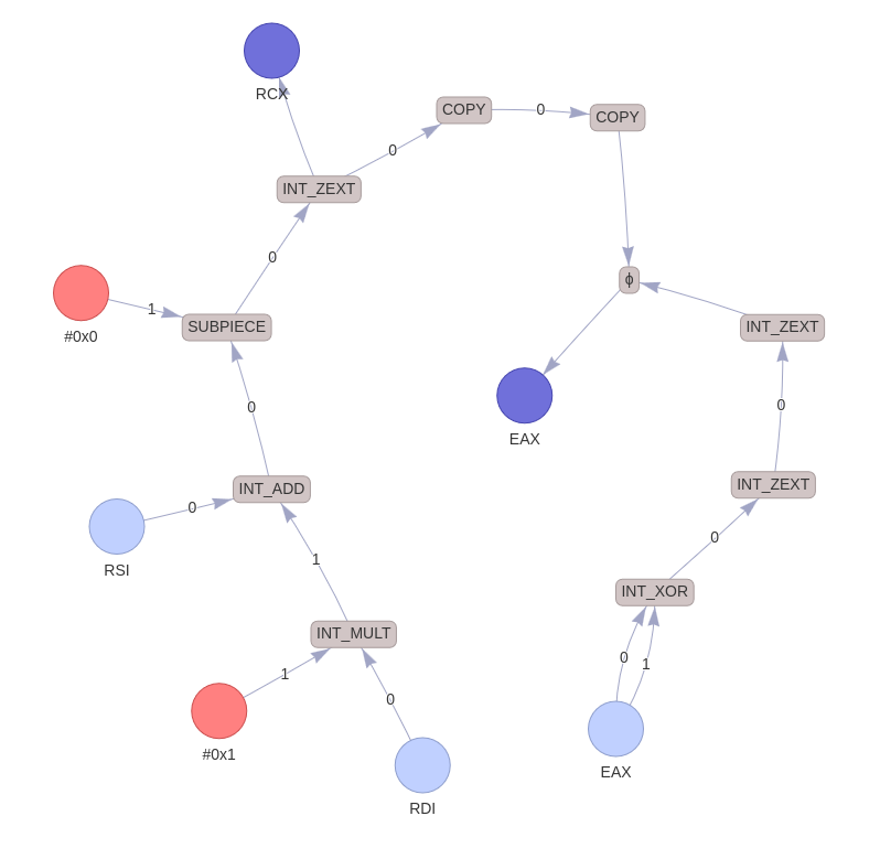
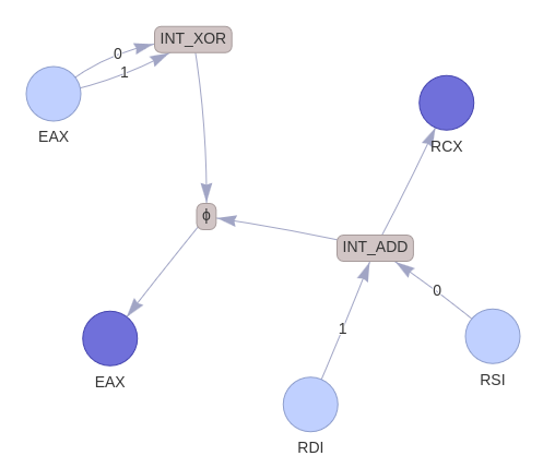
Dataflow before simplification. Source: original article.

Useless nodes gone. Instruction swap would not change this. Source: original article.

cdg html --dataflow-only test.o -o test_dataflow.html

cdg md --dataflow-only test.o > test_dataflow.md

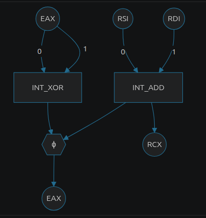
Same graph as markdown. Source: original article.

The Phi node still hides why EAX is 0 versus RDI+RSI. Dataflow alone is not enough. Add control-flow edges:

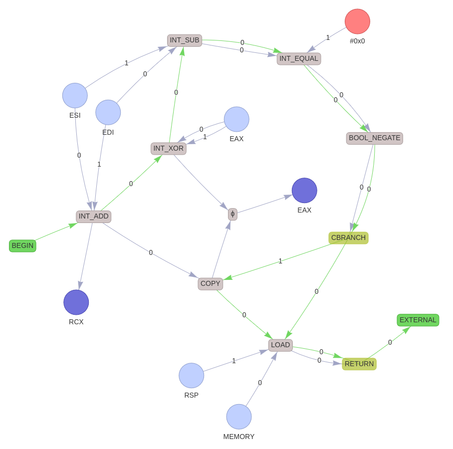
CDG: condition on EAX, return address load, EXTERNAL jump. Source: original article.

class NodeKinds(Enum):
    InputRegister = 0
    OutputRegister = 1
    Constant = 2
    Operation = 3
    Phi = 4
    ReadMemory = 5
    WrittenMemory = 6
    Begin = 7
    External = 8
    End = 9

Several memory nodes are allowed; no alias analysis, so addresses are not distinguished. Control-flow edges currently break permutation invariance. Hangouët flags a future format fix.

Kitchen table: Dataflow is who poured what into which bowl. Control flow is the order of the stove. For “is this the same recipe?” you want the bowls. For “which chef?” you want the order. Similarity wants bowls. Compiler fingerprinting wants order.

The Cisco Talos Dataset

Marcelli et al., USENIX Security 2022 / binary_function_similarity: 6 arch (x86/ARM/MIPS × 32/64), 8 compiler variants (gcc/clang × 4), 5 opt levels (O0–O3, Os). Functions via IDA. Train 256,625 / val 12,736 / test 522,003. Ten SOTA methods already scored on it.

Extracting 791k Graphs

LIEF for bytes at dataset offsets, then lift:

from pcode_graph.lief_importer import lookup_chunk
from pcode_graph.maker import make_graph_from_binary
from pcode_graph.translator import Translator

for arch, binaries in dataset_index.items():
    translator = Translator(arch)
    for binary_path, functions in binaries.items():
        binary = parse_binary(binary_path)
        for name, start, end in functions:
            code = lookup_chunk(binary, start, end)
            cdg = make_graph_from_binary(translator, code, start)
            output_path = compute_graph_path(dataset_dir, binary_path, name)
            output_path.write_bytes(pickle.dumps(cdg))

Wrong architecture on pypcode is surprising, not a clean error. They skipped 316 training-set labeling mistakes (Talos issue 39). Five-second timeout on analysis+graph+simplify drops 1.4% of functions. Parallel imap:

def run_in_parallel[P, R](
    function: Callable[[P], R],
    parameters: list[P],
    num_jobs: int | None = None,
    initializer: Callable = lambda: None,
) -> Iterator[R]:
    with multiprocessing.Pool(processes=num_jobs, initializer=initializer) as pool:
        for result in pool.imap_unordered(function, parameters):
            yield result

For operators: Default graph keeps all GPRs as outputs. For function semantics, keeping only the return register would shrink the graph and cut compiler-specific noise (flags, unused clobbers). Hangouët says that would have been smarter. Gadgets want the opposite: every flag.

Message Passing and Why Diameter Matters

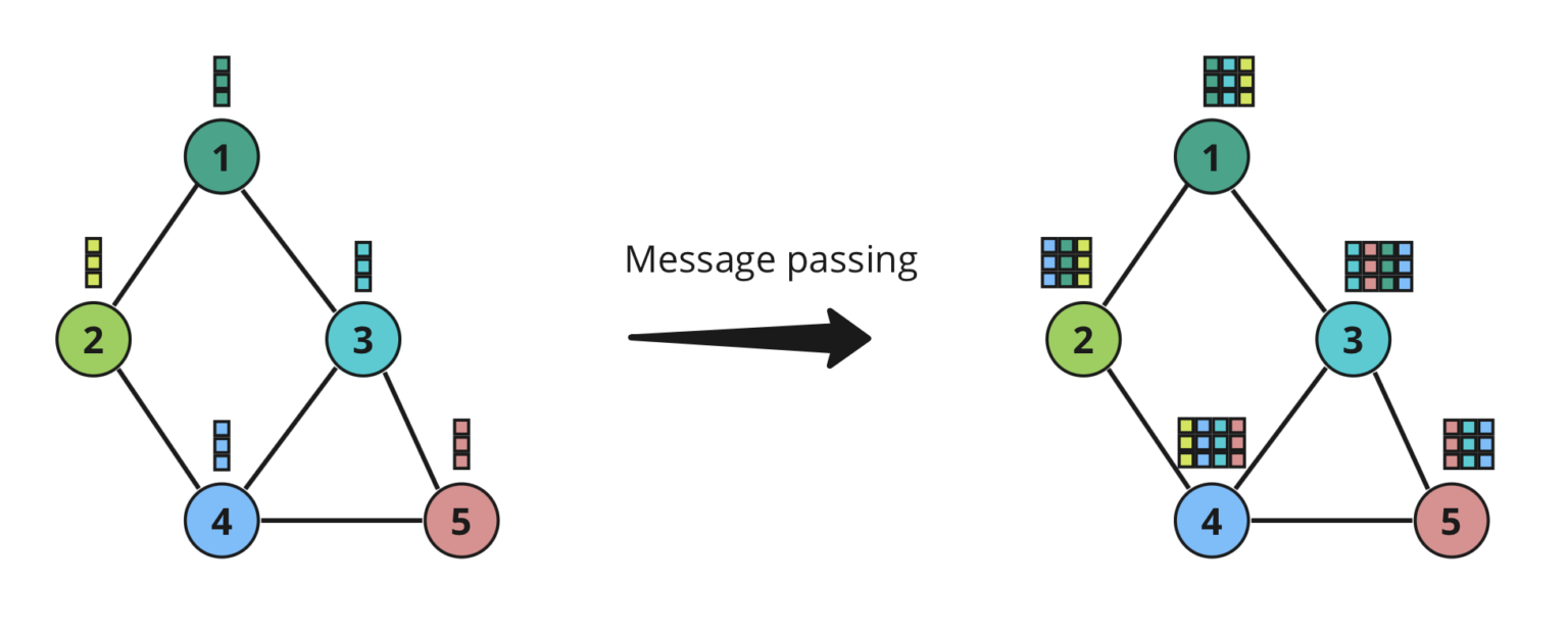
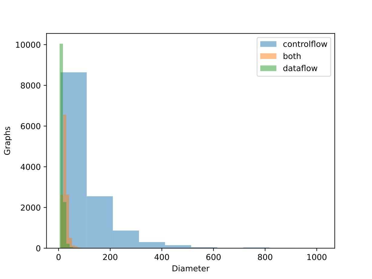
K convolution layers = K-hop neighborhood. Source: original article.

A GNN updates each node from its neighbors (message passing), then a readout pools nodes into one graph vector. Large diameter needs many layers. GNNs oversmooth past ~10 hops. So they want small diameter even on large functions. Validation diameters: control-only vs data-only vs both. Adding control slightly grows diameter; dataflow edges keep it in check.

Control vs data vs both. Source: original article.

GNN Architecture: GINE Baseline

No heroic search. GINE (Xu et al.) as a solid baseline, torch_geometric:

from torch import Tensor, relu
import torch
from torch_geometric.data import Data
from torch.nn import Dropout, ReLU, Linear, Module, ModuleList, Sequential
from torch_geometric.nn import GINEConv, global_add_pool, GraphNorm
from dataclasses import dataclass

@dataclass
class GNNConfig:
    readout_head_outputs: int = 256
    head_hidden: int = 256
    conv_hidden: int = 64
    conv_layers: int = 4
    feature_dropout: float = 0.5

class GINE(Module):
    def __init__(self, config: GNNConfig, node_features: int, edge_features: int):
        super().__init__()
        self.convs = ModuleList()
        self.norms = ModuleList()
        self.dropout = Dropout(config.feature_dropout)
        for i in range(config.conv_layers):
            dim_in = node_features if i == 0 else config.conv_hidden
            self.convs.append(
                GINEConv(
                    Sequential(
                        Linear(dim_in, config.conv_hidden),
                        ReLU(),
                        Linear(config.conv_hidden, config.conv_hidden),
                    ),
                    train_eps=True,
                    edge_dim=edge_features,
                )
            )
            self.norms.append(GraphNorm(config.conv_hidden))
        self.head = Sequential(
            Linear(config.conv_hidden * config.conv_layers, config.head_hidden),
            ReLU(),
            Dropout(config.feature_dropout),
            Linear(config.head_hidden, config.readout_head_outputs),
        )
    def forward(self, data: Data) -> Tensor:
        hs = []
        x = data.x
        for conv, norm in zip(self.convs, self.norms):
            x = conv(x, data.edge_index, data.edge_attr)
            x = relu(norm(x, data.batch))
            x = self.dropout(x)
            hs.append(global_add_pool(x, data.batch))
        return self.head(torch.cat(hs, dim=-1))

Loss: Supervised Contrastive, Not a Classic Triplet

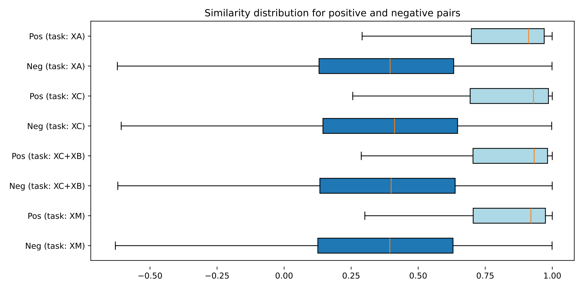
Embeddings are L2-normalized; similarity is a dot product. Instead of Siamese + triplet margin they use SupCon (Khosla et al., NeurIPS 2020):

similarity = (emb1 * emb2).sum().item()

def supcon_loss(features: Tensor, labels: Tensor, temperature: float):
    logits = matmul(features, features.T) / temperature
    logits_max, _ = logits.max(dim=1, keepdim=True)
    logits = logits - logits_max.detach()
    labels = labels.view(-1, 1)
    batch_size = features.shape[0]
    positive_mask = eq(labels, labels.T).float()
    self_mask = eye(batch_size, device=features.device)
    positive_mask = positive_mask - self_mask
    logits_mask = 1.0 - self_mask
    exp_logits = exp(logits) * logits_mask
    log_prob = logits - log(exp_logits.sum(dim=1, keepdim=True) + 1e-12)
    num_positives = positive_mask.sum(dim=1)
    mean_log_prob_pos = (positive_mask * log_prob).sum(dim=1) / clamp(
        num_positives, min=1.0
    )
    loss = -mean_log_prob_pos.mean()
    return loss

class SimilarityModel(Module):
    def __init__(self, num_node_features: int, num_edge_features: int):
        super().__init__()
        self.gnn = GNN(num_node_features, num_edge_features)
        self.optimizer = AdamW(self.gnn.parameters())
    def forward(self, graph_batch: Data) -> Tensor:
        z = self.gnn(graph_batch)
        return normalize(z, dim=1)
    def step(self, batch):
        emb = self(batch.graph)
        loss = supcon_loss(emb, batch.func_id, 0.07)
        self.optimizer.zero_grad()
        loss.backward()
        self.optimizer.step()

Tensors: Calling-Convention Registers, Not Raw EAX

graph_to_data maps registers through map_calling_convention_registers so arg0 / retval mean the same bit across x86_64 System V and AArch64 AAPCS. Same register can be both an argument and a return. Single-arch tasks can use hot-encoding via map_registers.

class Function(NamedTuple):
    bin_path: str
    func_name: str
    func_id: int
    graph: Data

class FunctionDataset(Dataset):
    def __init__(self, csv_path: Path):
        super().__init__()
        self.graphs = []
        architectures = set()
        ...
        self.register_mappers: dict[str, dict[str, Tensor]] = {}
        for arch in architectures:
            self.register_mappers[arch] = map_calling_convention_registers(arch)
    def __len__(self) -> int:
        return len(self.graphs)
    def __getitem__(self, index) -> Function:
        bin_path, arch, func_name, func_id, graph_path = self.graphs[index]
        graph = pickle.loads(graph_path.read_bytes())
        data = graph_to_data(graph, registers_emb=self.register_mappers[arch])
        return Function(bin_path, func_name, func_id, data)

SupCon wants several examples per class per batch. PK sampler: 4 samples × 16 functions:

SEED = 42
SAMPLES_PER_FUNCTION = 4
FUNCTIONS_PER_BATCH = 16

class BatchSampler(Sampler):
    def __init__(self, dataset) -> None:
        super().__init__()
        self.dataset = dataset
        self.rng = Random(SEED)
        self.num_batches = sum(1 for _ in self)
    def __len__(self) -> int:
        return self.num_batches
    def __iter__(self) -> Iterator[list[int]]:
        function_names = list(self.dataset.by_func_name.keys())
        self.rng.shuffle(function_names)
        samples: dict[str, list[int]] = {}
        for func_name in function_names:
            indices = list(self.dataset.by_func_name[func_name])
            if len(indices) >= SAMPLES_PER_FUNCTION:
                self.rng.shuffle(indices)
                samples[func_name] = indices
        while len(samples) >= FUNCTIONS_PER_BATCH:
            batch = []
            to_delete = []
            for func_name, indexes in islice(samples.items(), FUNCTIONS_PER_BATCH):
                batch += indexes[-SAMPLES_PER_FUNCTION:]
                if len(indexes) >= 2 * SAMPLES_PER_FUNCTION:
                    del indexes[-SAMPLES_PER_FUNCTION:]
                else:
                    to_delete.append(func_name)
            for k in to_delete:
                del samples[k]
            yield batch

Ping-pong GPU transfer so training stays GPU-bound:

def apply_to_batches(dataloader, func, device):
    previous_batch = None
    for batch in dataloader:
        next_batch = batch._replace(
            graph=batch.graph.to(device, non_blocking=True),
            func_id=batch.func_id.to(device, non_blocking=True),
        )
        if previous_batch is not None:
            func(previous_batch)
        previous_batch = next_batch
    func(previous_batch)

def train(device, csv_path):
    train_dataset = FunctionDataset(csv_path)
    train_data = DataLoader(
        dataset=train_dataset,
        pin_memory=device == "cuda",
        batch_sampler=BatchSampler(train_dataset),
        num_workers=16,
        persistent_workers=True,
    )
    model = SimilarityModel(train_dataset.node_features, train_dataset.edge_features)
    model.to(device)
    model.train()
    for e in range(config.num_epochs):
        apply_to_batches(train_data, model.step, device)

Still missing for a real pipeline: per-epoch val, TensorBoard, best-checkpoint save.

Results: Matching GMN on XM

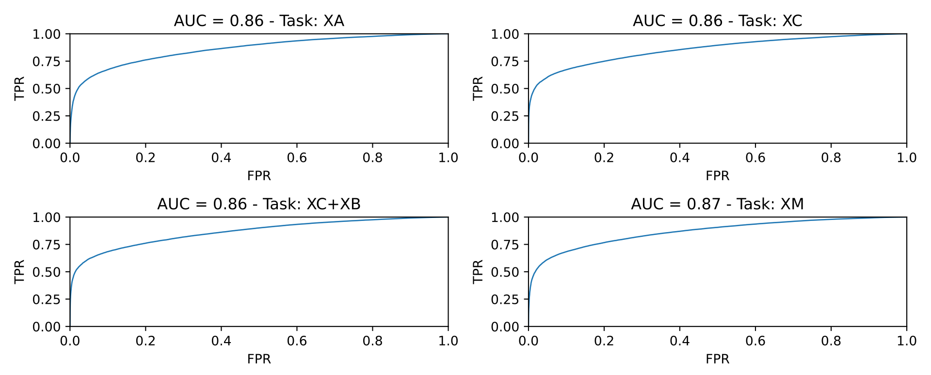
Pairs come from the paper. Score per pair, sweep threshold, ROC, AUC. Hardest task XM mixes arch, bitness, compiler and opt.

Testing ROC. Source: original article.

Positives and negatives separate. Source: original article.

Model	XC (same arch+bits)	XC+XB (same arch)	XA (same compiler)	XM (everything mixed)
GMN	0.86	0.87	0.86	0.87
GINE 4 layers + pcode_graph features	0.86	0.86	0.86	0.87

AUC vs GMN. 1.5% of larger functions dropped on timeout. Source: original article.

Not outstanding; you would not expect more without architecture search. It is a baseline that already ties the paper’s best graph matcher.

What a Reverse Engineer Actually Does with This

Patch diff: embed both builds, nearest-neighbor the functions that moved. Better than bindiff when the compiler flipped.
Malware family: cluster embeddings; a packer that only changes CFG noise should still sit near last week’s sample if dataflow survived.
Vulnerability search: embed a known-bad memcpy wrapper, query a firmware corpus.
ROP: keep flags as outputs; the graph of a gadget is the semantics of what it clobbers.
Not a decompiler. An embedding is a fingerprint, not C.

For operators: QuarksLab’s own 2019 Weisfeiler-Lehman kernel post is the non-neural cousin: same “semantic graph vs syntax” idea, cheaper at query time, weaker at XM. BSIM (Ghidra) uses High P-Code after decompiler SSA. pcode_graph here is closer to Raw P-Code plus homemade simplify. If you already run Ghidra decompiler, High P-Code MULTIEQUAL is a cleaner Phi than what this pipeline built from Raw. Hangouët is explicit the CFG-at-op-level may change.

Conclusion

pcode_graph turns binaries into semantic CDGs and, with a boring GINE + SupCon, matches GMN on Talos XM. Next: GATv2, DirGNN, real hyper-parameters, a graph format that stays permutation-invariant once control edges are back. Fork the MIT repo, send issues.

https://github.com/quarkslab/pcode_graph · pip install pcode_graph

Oversmoothing, in One Paragraph

Stack 20 GCN layers on a social graph and every node looks like the average of the graph: oversmoothing. Binary CDGs with long chains of int_zext / subpiece are the same trap. Four GINE layers plus jumping-knowledge style concat of every layer’s pooled state (the hs.append in forward) is how they keep early local ops in the embedding without 20 hops. If your functions are huge basic-block CFGs, this extractor’s op-level graph may have diameter worse than a BB graph. Measure before you copy conv_layers=4.

GMN versus GINE, Honestly

Graph Matching Networks compare two graphs jointly (cross-graph attention). GINE embeds each graph alone, then dots. Matching is stronger in theory for pairs you already have; embedding is what you need for a 500k-function index. Tying GMN’s AUC with a cheaper embedder is the practical win, even after dropping 1.4% timeouts. A production Sighthouse-style system wants the embedding.

What We Added

Kitchen recipes: -O0 vs -Oz as two cookbooks for one stew.
Operator notes: return-register-only outputs, gadget vs function modes, Talos mislabels.
RE shop uses: patch-diff, malware cluster, vuln search, ROP — and the High P-Code / BSIM cousin.
Oversmoothing and why four layers plus concat.

Key Takeaways

Same C, different -O, different ISA: mnemonic stats lie. Dataflow in 63 P-Code ops lies less.
Temporaries are edges. Simplify. Then add control flow, knowing it currently breaks permutation invariance.
Encode calling-convention roles, not EAX vs X0.
SupCon + PK batches (4×16) instead of one triplet at a time.
AUC 0.87 XM with 4 GINE layers, 1.4% timeouts dropped. Honest caveat vs GMN.
Library is MIT. Use it for diffs and corpus search, not as a magic decompiler.

Defensive / Lab Recommendations

If you ship firmware, assume someone will embed your functions against CVE PoCs. Strip and LTO change the graph; they do not make similarity impossible.
Obfuscation that only permutes instructions inside a block is weak against this extractor until control edges dominate.
MBA / VM-protect that changes dataflow will move the embedding. That is the ESANN use case: detect the obfuscator, then switch tools.
Validate on your own corpus before trusting Talos XM numbers. IDA function bounds in the dataset are a source of noise (they already skipped 316 mislabels).
Keep a 5s timeout. Pathological functions will stall SLEIGH forever.
Do not train on the test pairs. The paper already published them.

Original text: “From P-Code to GNN: extract binary code semantics” by Samuel Hangouët at Quarkslab. Library MIT: https://github.com/quarkslab/pcode_graph.